Unplanned production loss makes predictive vs preventive maintenance a cost decision about each machine’s failure modes. Retain justified calendar or run-hour tasks, and add condition-based prediction when a detectable precursor gives enough time to intervene and the avoidable loss exceeds the full monitoring cost.
Predictive vs preventive maintenance is best compared by the cost of a failure that each task can actually prevent. For a plant engineer weighing preventive vs predictive maintenance, the useful inputs are failure mechanism, production consequence, signal quality and response time. A calendar task suits a defensible service interval; a condition-based task suits deterioration that can be detected early enough to change the work order. An inexpensive, noncritical item may justify run-to-failure when its consequences are acceptable. Compare those choices over the same period, including installation, route labor, diagnosis and the failures that monitoring still misses.
Which equipment belongs on each side?
Assign a task to a failure mode before assigning a strategy to an entire machine class. A pump can retain scheduled lubrication while bearing deterioration receives a condition-based task; the two budgets can coexist.
NIST’s maintenance definitions distinguish time- or cycle-triggered preventive work from prediction-led intervention using condition observations. The broader national cost context is in maintenance accounting within digital manufacturing.
The following equipment examples apply the failure-mechanism and consequence approach described in NASA’s RCM guide and DOE’s maintenance-program discussion. They are starting points for an asset review, not blanket assignments.
| Approach | Candidate equipment or task | Dominant Failure Mode & Prevention | Cost question |
|---|---|---|---|
| Calendar or run-hour preventive maintenance | Consumable replacement or lubrication with a justified service interval | Wear or lubricant degradation addressed by the specified service task; retain the interval while checking that it matches duty. | Is the scheduled task preventing this mechanism, or replacing usable material without reducing the relevant risk? |
| Condition-based prediction | A production-critical motor, pump or gearbox with a detectable deterioration pattern | Developing bearing, alignment or lubricant problems addressed through suitable measurements, diagnosis and timely corrective work. | Can the team detect this mode and finish the intervention before functional loss? |
| Run-to-failure | An easily replaced, noncritical item whose loss leaves the required function available | Accepted component failure; contain its consequences with a suitable replacement arrangement or verified redundancy. | Does the complete consequence remain cheaper than a preventive or monitoring task, with safety and required functions protected? |
NASA’s section 2.2 retains interval work where wear, material change or an age–reliability relationship supports it. An unknown relationship between age and failure is a reason to investigate an appropriate condition technique; it is insufficient evidence for buying sensors across the fleet. DOE’s section 5.5 likewise makes equipment importance and downtime consequences part of the maintenance mix.
Rules of thumb for a signal worth paying for
Buy a measurement path only after checking its limits against the failure mode. The public ISO 17359:2018 abstract describes procedures for establishing a machine condition-monitoring programme; it supplies no machine-specific alarm value or financial threshold.
If a machine runs below 120 RPM, require a demonstrated measurement method for its duty before using vibration alerts to change PM. NASA’s September 2008 guide, section 6.3.2, identifies that low-speed range, complex machines, variable-speed operation and reciprocating machinery as difficult to monitor effectively. This is a qualification condition for the technique, rather than a universal speed cutoff for modern instruments.
If the thermal target is hidden, do not treat an external image as confirmation of its internal condition. NASA’s section 6.4.2 limits thermography to line of sight and identifies material, geometry and environmental error sources.
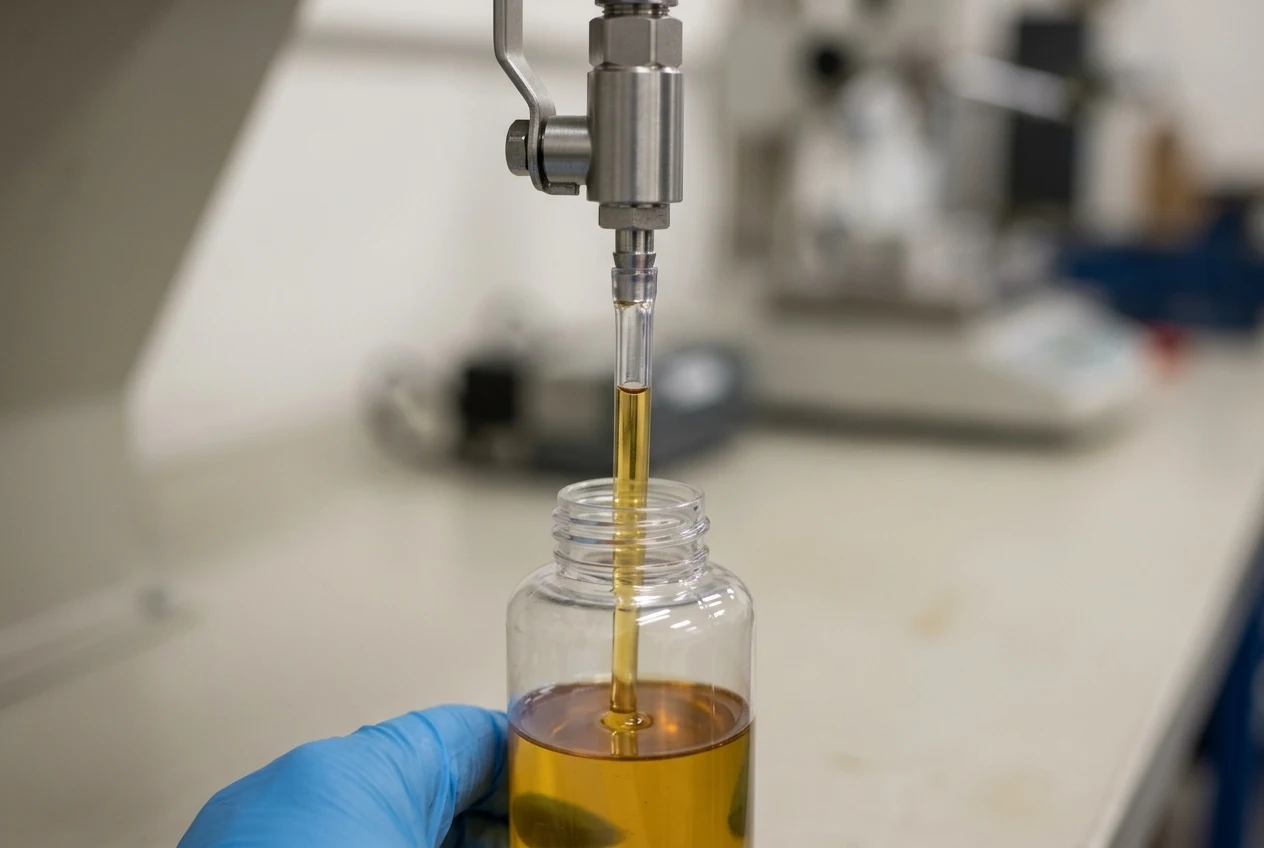
If oil samples cannot be collected consistently, fix the sampling route before using the trend to defer service. DOE’s section 6.3.1 specifies an active, low-pressure location before filtration, with repeat samples from the same point.
For vibration, mounting and acquisition quality matter alongside the number itself. DOE’s section 6.5.1 warns that general severity charts do not establish absolute failure boundaries. A generic alarm imported from a dashboard is therefore insufficient evidence to remove an existing task.

Will the warning arrive early enough to change the repair?
Condition monitoring needs enough usable warning for the next observation, technical review, parts availability, access and completed corrective work. A signal that arrives before failure can still arrive too late for the plant to benefit.
NASA’s section 5.2.2.2 recommends at least three monitoring points before expected failure to establish and confirm a trend, then shorter intervals as failure indications emerge. That guidance does not make three samples proof of remaining life or prescribe a monthly route for every asset.
For an illustrative timing check, assume the target mode offers 72 hours of usable warning, assume the next reading is at most 24 hours away, and assume the full response takes 36 hours after detection. Those assumptions leave some intervention margin. If the actual spare delay alone consumes the warning, increasing sample frequency cannot recover that delay; stock, repair access or another task must change. These are planning assumptions, not handbook thresholds.
Record who receives the warning and what action they can authorize. Include laboratory turnaround for sampled oil and the wait for an available crew. Where the precursor is unproven, keep the existing justified task while collecting evidence about detection and response.
What is the sensor-investment threshold?
Additional monitoring is financially defensible when its expected annual benefit is positive after all incremental costs are included. Compare it with the actual retained PM programme over the same accounting period.
For this comparison, use the following accounting identity:
Annual net benefit = downtime hours avoided × contribution lost per hour + unnecessary PM cost avoided − incremental annual monitoring cost.
Use contribution lost after avoidable variable costs, rather than gross sales per hour. Count only production that cannot be recovered through buffers, spare capacity or later scheduling. Keep restart scrap, emergency premiums and secondary damage in separate lines when the hourly contribution figure excludes them. Add each consequence once.
Every input below is an illustrative plant assumption. CU means arbitrary currency units; these figures are budget assumptions, not supplier prices or measured savings.
| Input | Assumption | Scope |
|---|---|---|
| Production-loss time avoided | 8 hours/year | Expected reduction relative to retained PM, after allowing for missed precursors and unnecessary alarm-driven stops |
| Contribution lost during that time | 1,500 CU/hour | Unrecoverable production contribution after avoidable variable costs |
| Unnecessary scheduled work avoided | 1,000 CU/year | Only tasks the evidence permits the plant to remove |
| Incremental monitoring cost | 9,000 CU/year | Annualized installation plus the net change in routes, analysis, training, maintenance and response costs |
| Route staffing within that cost | Two technicians for one hour per monthly route | Assumed access and staffing need; charged within the monitoring line, without counting it again |
Assumed annual net benefit = 8 × 1,500 + 1,000 − 9,000 = 4,000 CU/year.
The decision turns on those inputs. If a standby machine already prevents the assumed production loss, the benefit attributed to monitoring shrinks. If a warning cannot change the intervention, omit its claimed avoided hours. Annualize installed cost over the plant’s chosen evaluation life and financing assumptions; counting only a sensor purchase or one software invoice understates the commitment.
Which hidden costs can reverse the decision?
Route effort and imperfect diagnosis belong in the same comparison as hardware. When comparing condition monitoring vs preventive maintenance, retain the residual failure burden on both sides of the ledger.
| Cost factor | Plant record needed | Where it changes the decision |
|---|---|---|
| False alarms | Review time, repeat measurements and work orders closed without a relevant defect | Add diagnostic and response labor; subtract unnecessary stops from the downtime benefit. |
| Missed precursors | Failures without a usable prior warning, including modes the sensor cannot observe | Reduce credited avoided hours and retain the associated repair or damage burden. |
| Spare-part delay | Time from an actionable diagnosis to an available correct part and repair slot | Credit avoided loss only when warning can change the logistics or intervention. |
| Route labor | Travel, safe access, sample collection, identification, shipping and review | Include recurring technician effort even when acquisition hardware is already installed. |
| Sensor and data upkeep | Mounting checks, damaged cables, lost readings, baseline updates and analysis support | Include the continuing cost of a usable measurement history. |

Use one consistent convention: either net false-stop and missed-warning hours into the downtime benefit, as in the example, or show those loss costs separately. Doing both would count the same consequence twice.
For the next machine class, review the failure modes and work orders before extending the installation. Keep effective scheduled services, fund observable modes with an actionable warning, and accept run-to-failure only where the consequence review supports it. The industry section provides the broader manufacturing context; the sensor-install decision starts with this asset’s mechanism, response path and loss record.
Method and sources
Updated October 2026. NIST supplies the maintenance terminology; ISO’s public abstract supplies programme scope. NASA’s September 2008 facilities RCM guide supplies interval-selection and measurement-limit guidance, while DOE’s August 2010 O&M guide supplies sampling and vibration-limit context. The linked primary documents were retrieved on 19 October 2026. Equipment applications are engineering interpretations of those conditions. The accounting identity and explicitly assumed examples illustrate a plant decision; they do not forecast savings for another installation. The paid text of ISO 17359 is outside the evidence used here.