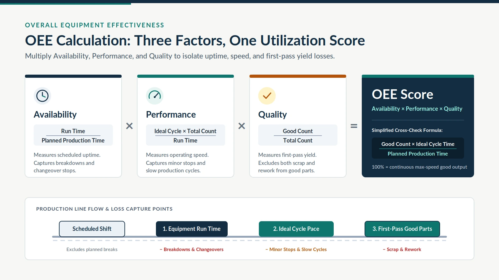
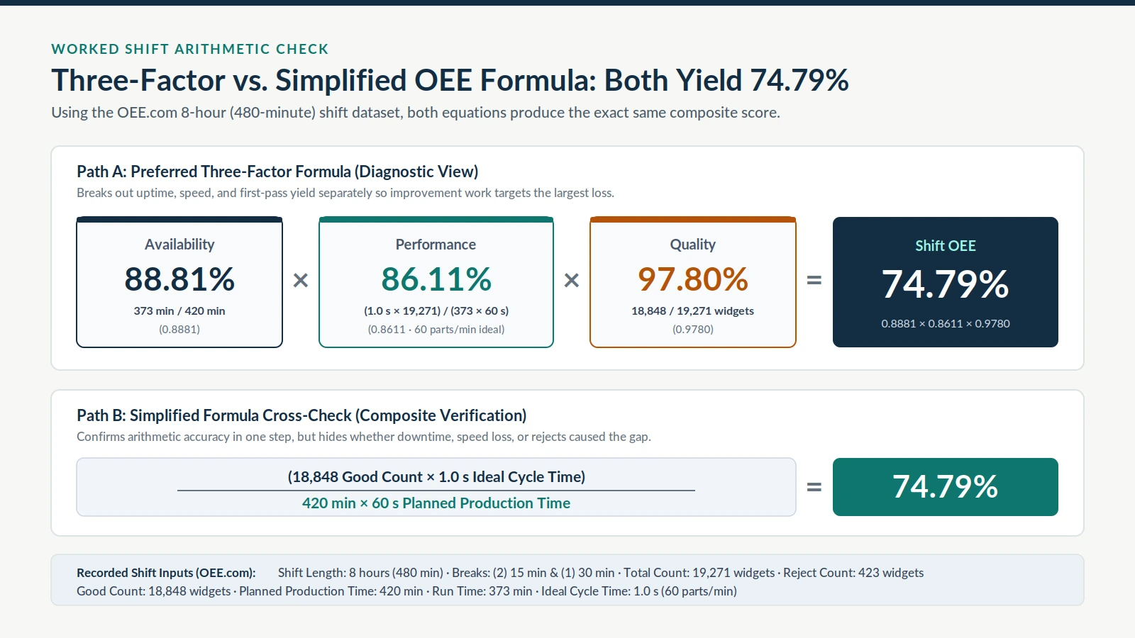
The standard OEE calculation multiplies three loss-focused factors: OEE equals Availability times Performance times Quality. Dividing Good Count times Ideal Cycle Time by Planned Production Time produces the exact same composite percentage, but the three-factor formula separates uptime, speed, and first-pass yield losses while keeping changeovers and breakdowns inside Stop Time.
Overall Equipment Effectiveness (OEE) measures how well manufacturing equipment is utilized compared to its full potential during the periods when it is scheduled to run, according to Wikipedia’s Overall equipment effectiveness entry. Within Total Productive Maintenance (TPM), OEE functions as a core metric for measuring equipment performance and guiding maintenance improvement, alongside broader factory-floor guides in our Industry section.
| OEE formula variant | Mathematical expression | Required shift inputs | Primary diagnostic role |
|---|---|---|---|
| Preferred three-factor formula | Availability × Performance × Quality | Planned Production Time (min), Stop Time (min), Ideal Cycle Time (s/part), Total Count (parts), Good Count (parts) | Isolates uptime, speed, and first-pass yield losses so teams target the largest constraint |
| Simplified cross-check formula | (Good Count × Ideal Cycle Time) / Planned Production Time | Planned Production Time (min), Ideal Cycle Time (s/part), Good Count (parts) | Verifies composite shift arithmetic as the ratio of Fully Productive Time to Planned Production Time |
What Is the Standard Formula for OEE Calculation?
The standard OEE calculation multiplies Availability, Performance, and Quality, whereas the simplified form divides Fully Productive Time by Planned Production Time. Both formulas evaluate equipment utilization against a theoretical 100% benchmark representing continuous operation at maximum speed producing only good products, a framework introduced in Seiichi Nakajima’s 1982 book TPM Tenkai.
In OEE.com’s calculation methodology (Vorne Industries), the simplest way to calculate OEE is as the ratio of Fully Productive Time to Planned Production Time, expressed as (Good Count × Ideal Cycle Time) / Planned Production Time. Substituting the definitions of Availability, Performance, and Quality cancels out Run Time and Total Count algebraically, which is why both equations always return the exact same composite percentage.
Although the simplified calculation is mathematically valid, OEE.com notes that it does not reveal how much capacity was lost to Availability, Performance, or Quality. For operational diagnosis, manufacturing teams use the preferred three-factor formula—OEE = Availability × Performance × Quality—and subdivide those three components into the Six Big Losses defined under TPM.
How Do You Calculate Availability in OEE?
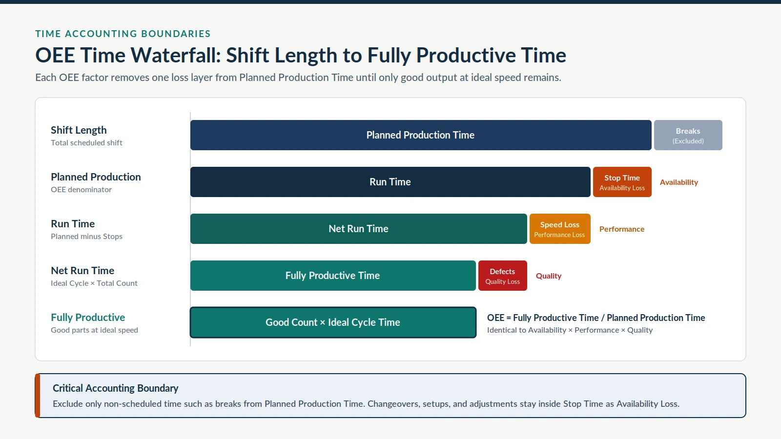
Availability is calculated by dividing Run Time by Planned Production Time, where Run Time equals Planned Production Time minus Stop Time. Availability isolates pure equipment uptime from Performance and Quality, starting from Planned Production Time after excluding only shift periods with no intention to run production, such as scheduled breaks.
Under OEE.com’s definitions, Stop Time includes all time when the manufacturing process was intended to be running but was not, covering both Unplanned Stops such as breakdowns and Planned Stops such as changeovers. Removing changeovers, setups, or waiting time from Planned Production Time instead of recording them inside Stop Time artificially inflates Availability and masks line bottlenecks.
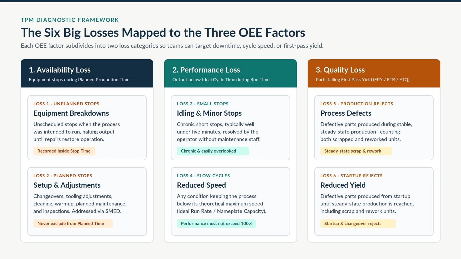
In the Six Big Losses framework, Planned Stops correspond to Setup and Adjustments, which covers setup, changeovers, major adjustments, tooling adjustments, cleaning, warmup time, planned maintenance, and quality inspections. Changeovers are typically the largest source of Setup and Adjustment time and can be reduced through a Single-Minute Exchange of Die (SMED) program, while equipment breakdowns are addressed through structured maintenance planning as examined in our guide to predictive vs preventive maintenance cost.
How Do You Calculate OEE Performance and Quality Factors?
Performance equals Ideal Cycle Time multiplied by Total Count divided by Run Time, while Quality equals Good Count divided by Total Count. Performance captures idling, minor stops, and slow cycles during Run Time, whereas Quality measures First Pass Yield by excluding both scrapped parts and parts requiring rework from Good Count.
Performance Calculation and the 100% Ceiling
In OEE.com’s formulation, Ideal Cycle Time is the fastest cycle time a process can achieve under optimal circumstances, so multiplying Ideal Cycle Time by Total Count yields Net Run Time—the fastest possible time to manufacture those parts. Teams that track speed in parts per minute rather than seconds per part can use the equivalent rate equation: Performance = (Total Count / Run Time) / Ideal Run Rate.
Performance should never exceed 100%. When a shift report shows Performance above 100%, OEE.com notes that the result usually indicates Ideal Cycle Time is set too high rather than genuine over-speed production.
Performance captures two of the Six Big Losses: Idling and Minor Stops and Reduced Speed. Idling and Minor Stops covers short stops—typically well under five minutes—that operators resolve without maintenance personnel; because the underlying issues are often chronic, operators can become blind to their cumulative impact. Reduced Speed covers any condition that prevents equipment from running at its theoretical maximum speed, also known as Ideal Run Rate or Nameplate Capacity, while the process is running.
Quality Calculation and First Pass Yield
Quality measures Good Units produced as a percentage of Total Units produced and is commonly referred to as First Pass Yield (FPY), First Time Right (FTR), or First Time Quality (FTQ). Good Parts include only units that successfully pass through the manufacturing process on the first try without needing rework.
Quality captures the final two categories of the Six Big Losses: Process Defects and Reduced Yield. Process Defects accounts for defective parts—both scrap and rework—produced during stable, steady-state production, whereas Reduced Yield accounts for defective parts—both scrap and rework—produced from equipment startup until steady-state production is reached.
| OEE factor | Six Big Losses category | Typical shop-floor events | Required accounting rule |
|---|---|---|---|
| Availability | Unplanned Stops | Equipment breakdowns and unscheduled failures | Subtract from Planned Production Time as Stop Time (minutes) |
| Availability | Setup and Adjustments (Planned Stops) | Changeovers, tooling adjustments, cleaning, warmup, planned maintenance, quality inspections | Keep inside Planned Production Time and record as Stop Time (minutes); never exclude as breaks |
| Performance | Idling and Minor Stops | Chronic short stops well under five minutes resolved by operators without maintenance staff | Captured automatically through the gap between Run Time and Net Run Time |
| Performance | Reduced Speed | Running below Ideal Run Rate or Nameplate Capacity during active production | Benchmark against optimal Ideal Cycle Time; audit whenever Performance exceeds 100% |
| Quality | Process Defects | Defective parts produced during steady-state production | Exclude both scrapped and reworked parts from Good Count (parts) |
| Quality | Reduced Yield | Defective parts produced from startup until steady-state production | Exclude both startup scrap and startup rework from Good Count (parts) |
Why Is the Three-Factor OEE Calculation Preferred Over the Simplified Formula?
The three-factor OEE calculation is preferred over the simplified formula because it exposes whether lost capacity stems from equipment stops, slow cycles, or defective parts. A single composite OEE percentage cannot warn a plant when gains in one factor are offset by harmful losses in another.
OEE.com illustrates this risk with a two-week comparison: most companies would not want to increase Availability by 5.0% at the expense of decreasing Quality by 4.5%. Looking only at the simplified composite number hides that deterioration in first-pass yield, whereas tracking Availability, Performance, and Quality side by side flags the defect spike immediately.
Scope boundaries matter just as much as factor visibility. While the performance of a particular product can be determined from OEE data, OEE cannot be calculated for an individual product because all downtime and availability losses would have to be correlated to specific products. Keeping OEE anchored at the machine or production-line level—aligned with job-linked records described in what digital manufacturing means on the factory floor—prevents distorted downtime allocation.
How Does a Step-by-Step OEE Calculation Example Work on a Production Shift?
On OEE.com’s reference 8-hour (480-minute) production shift, subtracting scheduled breaks gives 420 minutes of Planned Production Time and 373 minutes of Run Time. Multiplying Availability (88.81%), Performance (86.11%), and Quality (97.80%) yields 74.79% OEE, matching the simplified formula to the second decimal place.
The recorded shift dataset from OEE.com consists of an 8-hour (480-minute) Shift Length, scheduled Breaks of two 15-minute breaks and one 30-minute break, a Total Count of 19,271 widgets, a Reject Count of 423 widgets, and an Ideal Cycle Time of 1.0 seconds per widget (an equivalent Ideal Run Rate of 60 parts per minute). Working through the factors sequentially produces the following shift breakdown:
| Calculation step | Formula applied | Shift values with units | Result |
|---|---|---|---|
| Shift Length | Recorded shift schedule | 8 hours | 480 minutes |
| Scheduled Breaks | Recorded non-scheduled breaks | (2) 15 minutes and (1) 30 minutes | Excluded from Planned Production Time |
| Availability | Run Time / Planned Production Time | 373 minutes / 420 minutes | 0.8881 (88.81%) |
| Performance | (Ideal Cycle Time × Total Count) / Run Time | (1.0 seconds × 19,271 widgets) / (373 minutes × 60 seconds) | 0.8611 (86.11%) |
| Quality | Good Count / Total Count | 18,848 widgets / 19,271 widgets | 0.9780 (97.80%) |
| OEE (three-factor) | Availability × Performance × Quality | 0.8881 × 0.8611 × 0.9780 | 74.79% |
| OEE (simplified check) | (Good Count × Ideal Cycle Time) / Planned Production Time | (18,848 widgets × 1.0 seconds) / (420 minutes × 60 seconds) | 74.79% |
Notice how both calculation paths converge on 74.79% OEE, yet the three-factor breakdown immediately shows that Performance (86.11%) and Availability (88.81%) account for far more lost capacity than Quality (97.80%). Converting time into consistent units—multiplying 373 minutes by 60 seconds when Ideal Cycle Time is expressed as 1.0 seconds—prevents unit-mismatch errors in both hand calculations and spreadsheets.
How Do You Set Up an OEE Calculation Sheet in a Spreadsheet?
An accurate OEE calculation sheet separates raw shift inputs from calculated factor columns and computes both the three-factor formula and the simplified formula on every row to verify arithmetic. Locking Planned Production Time to exclude only scheduled breaks and flagging Performance above 100% keeps shift reports consistent.
To keep spreadsheet tracking auditable across shifts, structure one row per machine or production line per shift rather than trying to compute separate OEE scores per product. Keep time units consistent across all columns—converting minutes to seconds when Ideal Cycle Time is entered in seconds—and enforce the following column layout:
| Spreadsheet column | Column type | Definition or formula | Built-in audit check |
|---|---|---|---|
| Shift Length (min) | Raw input | Scheduled shift duration in minutes | Verify against plant shift calendar |
| Scheduled Breaks (min) | Raw input | Time with no intention of running production | Allow scheduled breaks only; never place changeovers here |
| Planned Production Time (min) | Formula | Shift Length minus Scheduled Breaks | Must remain strictly positive for every scheduled shift |
| Stop Time (min) | Raw input | Sum of Unplanned Stops (breakdowns) and Planned Stops (changeovers, setups, adjustments) | Confirm all changeover and planned maintenance minutes during scheduled production are included |
| Run Time (min) | Formula | Planned Production Time minus Stop Time | Cannot be negative or exceed Planned Production Time |
| Ideal Cycle Time (s/part) | Reference input | Fastest cycle time achievable under optimal circumstances | Re-audit immediately if Performance exceeds 100% |
| Total Count (parts) | Raw input | All parts produced during the shift | Must include good parts, scrap, and rework |
| Reject Count (parts) | Raw input | Scrapped parts plus parts requiring rework | Follow First Pass Yield; do not credit reworked units as good |
| Good Count (parts) | Formula | Total Count minus Reject Count | Must be less than or equal to Total Count |
| Availability (%) | Formula | Run Time / Planned Production Time | Pure uptime ratio isolated from speed and quality |
| Performance (%) | Formula | (Ideal Cycle Time × Total Count) / (Run Time × 60) | Flag any row above 100% as an Ideal Cycle Time error |
| Quality (%) | Formula | Good Count / Total Count | Matches First Pass Yield (FPY / FTR / FTQ) |
| OEE Three-Factor (%) | Formula | Availability × Performance × Quality | Primary operational metric for loss prioritization |
| OEE Simplified Check (%) | Formula | (Good Count × Ideal Cycle Time) / (Planned Production Time × 60) | Must equal OEE Three-Factor on every shift row |
When the three-factor column and the simplified check column match on every row, arithmetic and unit-conversion errors are ruled out immediately. From there, comparing Availability, Performance, and Quality across shifts shows whether the next improvement project should target SMED changeover reduction, chronic minor stops, slow cycles, or startup yield losses.